Local Government Transparency Scores: Methodology
This document describes the methodology used to create the transparency indicators for the Government Transparency Project. We use webscraping and machine learning models to estimate whether a given website has the following transparency indicators:
- Meeting Agendas (AGD): Posted agendas for regular meetings of the main policy-making body (e.g. the city council or its equivalent) of the local government.
- Budgets (BDG): Town budget.
- Public Bids (BID): Posted information about bids for contracts to provide goods or services for the city.
- Comprehensive annual financial reports (CAFR): Posted annual financial reports.
- Meeting Minutes (MIN): Posted minutes for regular meetings of the main policy-making body (e.g. the city council or its equivalent) of the local government.
- Public Records Requests Information (REC): Description or form that states how to obtain public records.
Below, we describe the specific data and algorithms used to generate the indicators included on the transparency report cards.
Data
Training Sample
The sampling frame for our training sample are all US towns with a population greater than 1000, as measured by the 2010 census. Specifically, we use census data on “incorporated places” as our target population, which amounts to 39548 administrative units.
Our training sample consists of manually labeled indicators from 818 towns. The sample is broadly representative of the population of towns with populations greater than 1000 in the United States, with some over-representation of particular states such as New York and Texas.1 Because of the over-representation of towns from a few states, the typical town in our training sample is larger in population than the typical town in the US, but the distributions overlap substantially. This comparison is visualized in Figure 1.
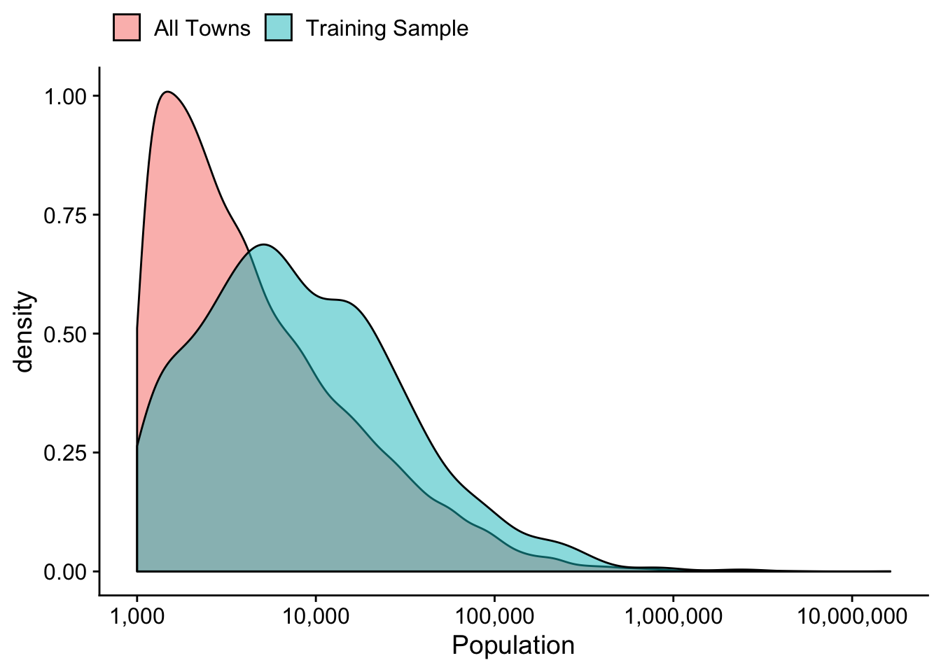
Figure 1: Distribution of Town Population in Training Sample and All US Towns with population greather than 1000.
The training sample towns represent 49 distinct states. The geographic distribution of the training sample by state is depicted in Figure 2.
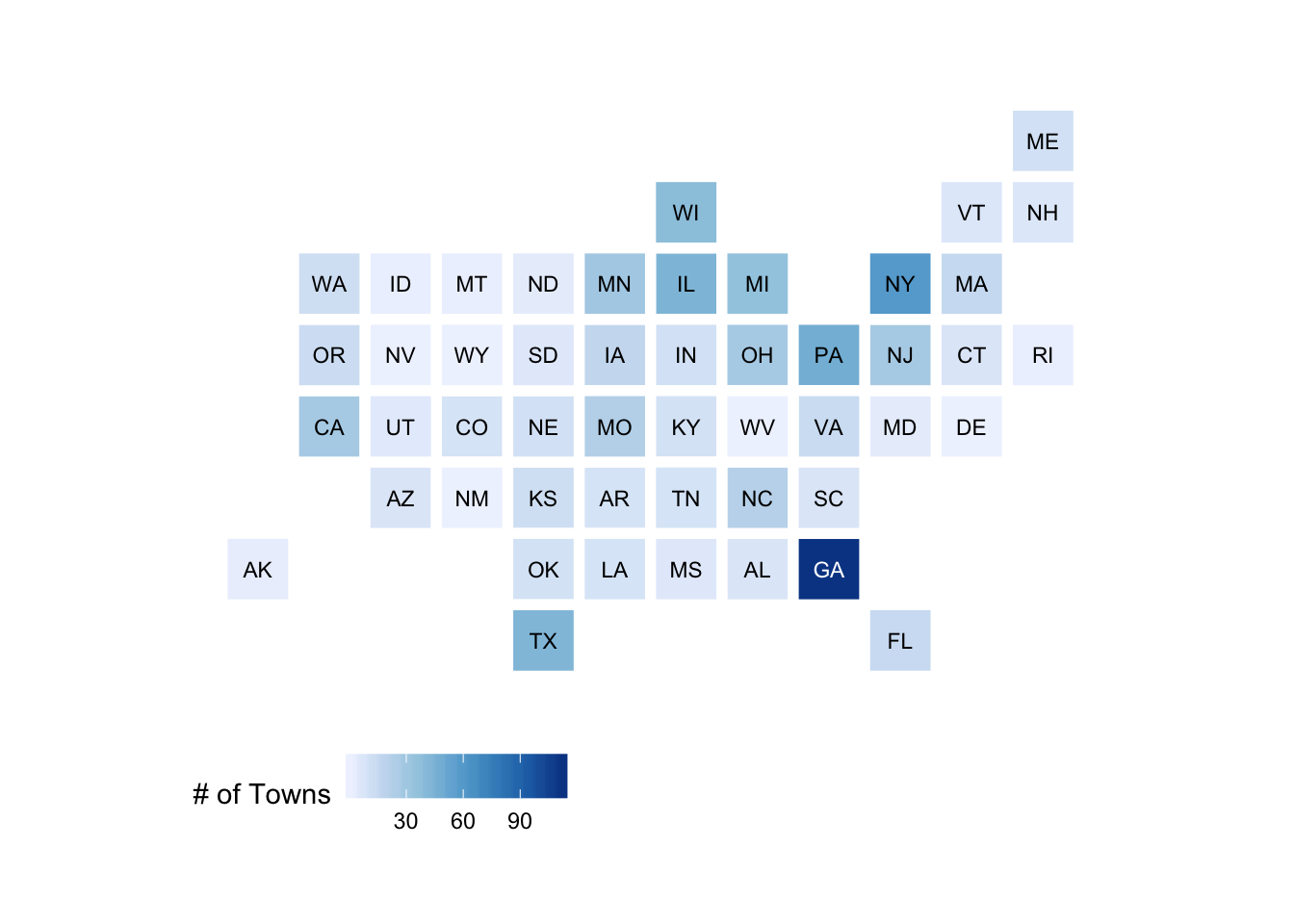
Figure 2: Geographic Distribution of Towns in the Training Sample
Scraping Websites
To obtain the text data used to train the model or to label a website, we use the Python crawling framework Scrapy. Specifically, we crawl each website up to a depth of 2, with a maximum limit of 500 pages, and save the HTML of each crawled page. This depth limit means that in addition to the home page (level 0), we crawl pages that are linked from the home page (level 1), and pages that are linked from those pages as well (level 2). Finally, we impose a limit of 500 pages to keep the data of manageable size.
Creating a Document Term Matrix
For use in the classification model, we concatenate selected text from all pages of a given website and transform the text into a document term matrix (DTM). Specifically, from each scraped page we extract the (1) text in the title of the page, (2) the text in all links of each page, and (3) the full text of the page itself. Each set of text (i.e. title text, page text, or link text) is concatenated into a separate text string.
We then transform and pre-process each string of text into a document term matrix using the R package Quanteda(Benoit et al. 2018). Specifically, we remove punctuation, symbols, hyphens, and a list of common stop words. After this pre-processing, we convert the string to a document-term matrix of unigram counts. When creating the training set, we remove any token that does not occur in more than 10% of the websites.
After pre-processing and conversion is completed, the title text DTM, the link text DTM, and the page text DTM are combined into a single matrix, though columns denoting the term counts from each of the tree text types (links, titles, and pages) are kept in separate columns. The DTM generated from our training sample using these procedures has 13311 columns.
Classification Model
To classify websites we use a random forest(Breiman 2001) model combined with a feature selection pre-processing step. The feature selection step reduces the dimensionality of the of the full DTM considerably and improves the predictive performance of the random forest model.
Feature Selection
The feature selection step relies on calculating a bivariate correlation between the transparency indicator and each column of the document term matrix. Specifically, we compute the information gain between the indicator and each column of the document term matrix, which is a univariate measure of association between the two variables.. We then rank the columns with respect to information gain and keep the top \(p\)% percent of the variables, where \(p\) is chosen via cross-validation.
The proportion of terms retained for each model are as follows:
- AGD: 0.11
- BDG: 0.57
- BID: 0.27
- CAFR: 0.13
- MIN: 0.2
- REC: 0.12
Random Forest Model
After weakly correlated variables are pruned from the document term matrix via the feature selection step, we use a Random Forest model to predict the transparency indicator. Specifically, we use the implementation in the ranger(Wright and Ziegler 2017) package, which is optimized for speed. Each model is an ensemble of 500 different classification trees. When constructing individual trees, Random Forest models use only a random subset of both the training sample and the predictors (post-feature selection). Specifically, each tree uses a random sample (with replacement) of 0.9 of the number of units in the training sample. The predictors used in each tree are also a random sample, where the number of predictors retained is equal to the square root of the total number of predictors in the post-feature selection DTM.
The only model hyper-parameter that is tuned performed is the proportion of variables to retain via the feature selection step described above. We use cross-validation on the combined feature selection and random forest procedures to choose an optimal proportion of variables to retain.
To understand what aspects of the website are used when predicting each label, we computed the permutation importance of each column of the DTM. Specifically, we permute each column of the DTM and calculate the increase in prediction error. This statistic provides one measure of the relative importance of each unigram count from the website. The results for the 6 models can be found in Figure 3. Unsurprisingly, the most predictive unigrams tend to be the labels themselves, such as “budgets”, “minutes”, etc.
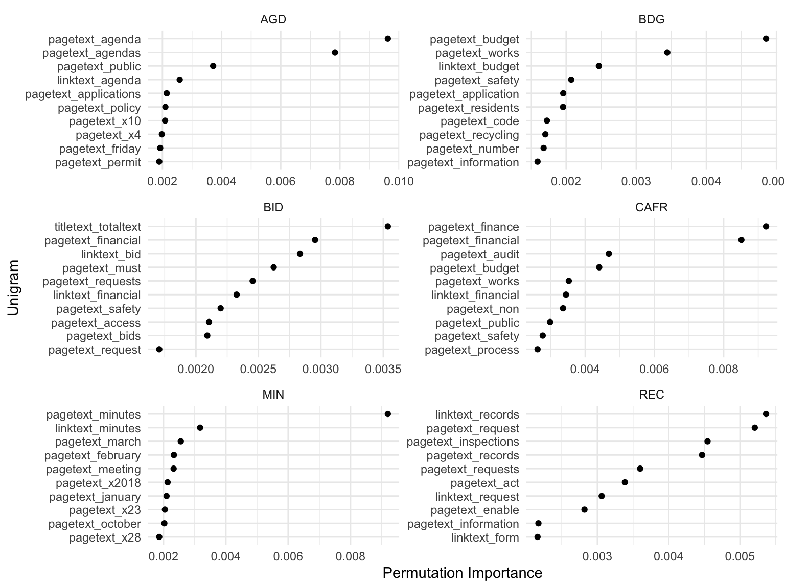
Figure 3: Permutation Importance. Shows 10 columns of the document term matrix that have the highest permutation importance.
Out of Sample Performance
To estimate performance of the model, we use cross-validation. Specifically, we do 5-fold cross-validation, repeated 10 times. Table 1 reports the results for overall accuracy, positive predictive value, and negative predictive value. Positive predictive value is defined as the proportion of correct labels among sites labeled as having the indicator, while negative predictive value is the proportion of correct labels among sites labeled as not having the indicator.
| label | Accuracy | Negative Predictive Value | Positive Predictive Value |
|---|---|---|---|
| REC | 0.77 | 0.76 | 0.79 |
| MIN | 0.84 | 0.65 | 0.88 |
| CAFR | 0.80 | 0.79 | 0.81 |
| BID | 0.81 | 0.82 | 0.80 |
| BDG | 0.82 | 0.76 | 0.85 |
| AGD | 0.85 | 0.79 | 0.88 |
Benoit, Kenneth, Kohei Watanabe, Haiyan Wang, Paul Nulty, Adam Obeng, Stefan Müller, and Akitaka Matsuo. 2018. “Quanteda: An R Package for the Quantitative Analysis of Textual Data.” Journal of Open Source Software 3 (30): 774. https://doi.org/10.21105/joss.00774.
Breiman, Leo. 2001. “Random Forests.” Machine Learning 45 (1): 5–32.
Wright, Marvin N., and Andreas Ziegler. 2017. “ranger: A Fast Implementation of Random Forests for High Dimensional Data in C++ and R.” Journal of Statistical Software 77 (1): 1–17. https://doi.org/10.18637/jss.v077.i01.
These states were over-sampled because external validation data exists for towns in these states. This external validation data will be used to assess the overall validity of the transparency score.↩︎
F. Daniel Hidalgo
Associate Professor of Political Science
I'm a political science professor at MIT, specializing in electoral politics in Latin America.